In Part I of this blog series, we introduced you to an alternative to conventional ERP forecasting systems. In Part II, let’s examine how forecasting holds the inventory of a product versus Shippers Solutions’ suggested strategy.
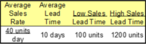
Let’s say on average a product sells at the rate of 40 units per day over the course of a year. However, both the rate of sales rate and the lead time is subject to chaotic fluctuations. From a statistical perspective, the variability is meaningless, that is, it is not indicative of any trend. During the 10 days it takes to get more, sales have peaked at 1200 units and have been as low as 100. Occasionally, the supplier delivers as much as 2 days late.
The users of the ERP system chose a reorder point of 21 days’ worth of stock, thinking that since it may take 12 days to get more inventory, that leaves an extra 9 days’ worth of safety stock to protect against heavy sales. This is a thoughtful and logical decision that, because of forecasting, just doesn’t work.
The ERP system uses its forecasting algorithm to calculate how long the current inventory will last. Even when demand changes do not represent a trend, the forecast produced by the ERP system fluctuates up and down.
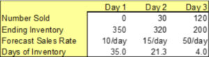
If sales have been slow recently, the forecast will be low, let’s say only 10 per day. If there are 350 units in stock at the end of the first day, the ERP computes 35 days’ worth of inventory in stock. No order is placed because inventory hasn’t yet dropped to 21 days’ worth. When sales pick up on Day 2, the forecasted sales rate might increase to 15 per day. Still, no order is placed because the number of calculated days of inventory remains above the threshold of 21 days. Day 3’s large sale of 120 units raises the forecasted consumption rate up to 50 per day. If so, the days-on-hand drops precipitously to 4. An order is immediately placed. Sadly, the company is unlikely to get delivery before running out because the normal consumption in the 10-day supplier response is 400 units.
If you’d like to see this more visually, please click here to see a short video on the subject. I call this effect Submarining.
After the stock out occurs, the person responsible for inventory availability rightly concludes that the safety stocks must have been insufficient and raises them by changing the reorder point for this, or maybe all products, to say 30 days’ worth. Inventory on hand increases. The trial-and-error pattern is repeated until shortages are reduced to what feels like an acceptable level. Acceptable means, not causing more work than the staff has time for in a busy day.
The quantity ordered at a time is another major factor that determines the level of inventory. In very many ERP implementations the order quantity is based on an old rule which predates the ERP system.
For example, the order quantity could have been set to 40 days’ worth. Back when the rule was established, there were only so many people in the Purchasing Department. Together they could only place purchase orders for so many products per day. They simply divided the number of products they had to manage by the number the department could handle in a day. The result was a decision to buy 40 days’ worth. Without adding manpower, they simply couldn’t get around to each product more often.
The capability of the ERP system to order each item every day does not guarantee that the old rule is reconsidered. After all, it is difficult enough to implement an ERP system without also questioning every procedure that works fine as is.
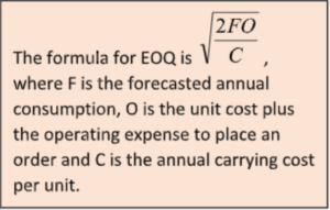
Alternately, the computing power of the ERP system can be used to recalculate the Economic Order Quantity (EOQ) for each item when it reaches its reorder point. This supposedly optimal purchase quantity is designed to minimize both the costs of placing orders and carrying inventory. As orders get larger, the inventory on hand is bigger for longer which raises the carrying cost of the inventory. As orders get smaller, they become more numerous, increasing the costs associated with placing orders.
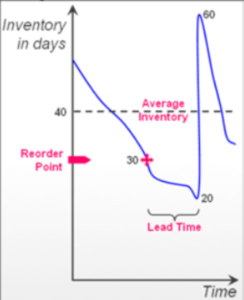
Average inventory on hand is simply the reorder pointless consumption during the lead time plus ½ the order quantity. (See the diagram. If the example product above is representative of the rest of the products, then the number of days of on-hand inventory we calculate applies overall. (Since we are calculating inventory levels in terms of the average number of days it will last, the outcomes are comparable across the company. If your lead time is longer or variability greater, your inventory in days will increase.) Let’s compare the differences between the on-hand inventory levels for your conventional circumstances and Shippers‘ improved model.
The flaw of EOQ is based on the assumption that the cost of placing an order is fixed, which is no longer true. EOQ was put forth back in 1913, long
before computers. Back then, placing more orders meant paying more people in the typing pool. Now, the ERP system can easily order each item every day. With the underlying assumption of EOQ debunked, ordering batches provides generic disadvantages. (Batches are still useful in special cases, for example, to reduce inbound freight costs, to earn a quantity discount, to buy-in before a price increase, or to meet supplier-imposed order multiples or minimum order quantities.) With smaller order quantities, carrying costs and investment in inventory are reduced while availability is improved by simply having the computer order what is consumed every day.
At Shippers’, when we manage pools of inventories used to buffer against shortages, we include both what is on hand plus goods that have been ordered but not yet received – the inbound inventory. To protect the availability, the buffer should have 1200 units to handle the high consumption we have already seen. (See the first table above.) Add to that, 2 days’ worth or 80 units to protect against late delivery. So, the buffer size is 1280 units. Divide this figure by the average consumption of 40/day to get the buffer size of 32 days’ worth. Remember, our buffers include inbound, so on average there are 400 units inbound (average consumption of 40 units per day × the 10 days it takes to receive the goods, again on average). That leaves 22 days’ worth on-hand. Of course, there will be fluctuations based on the big swings in demand but that’s the average. Interesting, huh? It’s about half what your expensive ERP holds on-hand. Even if you take advantage of volume discounts, buy in minimum order quantities, and in order multiples, this order batching only raises the days on-hand a little bit.
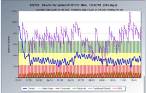
Bottom line: managing to flow instead of by forecasts improves availability with around half as much inventory. Here’s a picture of a typical example. The purple dotted line is how inventory fluctuated when managed by the ERP system. The solid blue line is what would have happened with the exact same consumption pattern using SSCo’s flow management approach. Want some money back?