
All companies that hold inventory are subject to obsolescence. It can be that the product exceeds its shelf life or that another product becomes preferred (expired market life). However, practically speaking, obsolescence usually occurs due to the loss of a customer for the product. Hope springs eternal that a new customer will be discovered or that the old customer will return. Either way, until then, dead inventory is absolutely worthless. In the 3rd and final part of this series we will share another conventional ERP forecasting approach versus Shippers’ buffer model comparison to illustrate how obsolete inventory is managed.
Conventionally, obsolete inventory is an unwanted and costly portion of total inventories. Although, in many companies it represents much more, to give the benefit of the doubt to the conventional approach, we will assume dead inventory is only 10%. So, for this factor, we must add another 4 days’ worth (40 days × 10%) to average inventory making it 44 days’ worth.
Since Shippers Solutions’ approach holds far less inventory (22 days versus 40 days), there is less to get stuck with; which means we are proportionally less exposed to dead inventory. Our expected obsolescence is more like 2 days’ worth, again, half conventional dead stock.
A quantity of each item that is equivalent to obsolete inventory is typically tied up in products which are now moving more slowly than expected when they were purchased. A customer for these products might have been lost. (Perhaps because the company ran out one time too many?) Other customers will use up the excess but not for a long time. Using ERP, the opposite of the stock-out scenario described in Part II applies here to create surpluses. When sales have been unusually robust a high forecast results. Reorders are placed too soon and for too much.
Say the high forecast is 75 units per day. Using the 30-day reorder point, the ERP system suggests an order when on hand inventory is at 2,200 units. (The calculation is 2,200 units on-hand / 75 units per day = 29.3 days on-hand.) The problem is that future sales are far more likely to be 40 units per day. Using the same formula, the ERP orders when 55 days’ worth are in stock. To make matters worse, the software also recalculates the reorder quantity by multiplying its 75 units per day forecast by the standard 40-day order quantity, boosting the amount ordered to 3,000 units. If demand reverts to normal, 400 units will be sold during the 10 days of lead time, reducing the 2,200 units to 1,800 by the time the order for 3000 arrives. Peak inventory is then 4,800. Divide that by the normal consumption rate to get 120 days’ worth. Voilà! Surplus inventory.
If you’d like to see this more visually, please click here to see a video on the subject. I call it Ski Jumping.
It is unlikely that forecast driven surpluses are less than 4 days’ worth (4 weeks may be more like it). In all, total inventory for our conventional example is 40 days for the normal items plus 4 days for the dead inventory plus 4 more days for surpluses caused by forecasting and another 2 days for surpluses due to lost customers.
Total ERP inventory = 50 days’ worth
Shippers Solutions’ response to heavy consumption is seen in our approach. Since reorders are placed daily for the amounts sold, temporarily heavy sales pulls on-hand inventory lower – inbound inventory increases as a proportion of the buffer. Likewise, slower than average sales increase the on-hand amount as less is purchased and still inbound. These two factors offset each other causing no net surplus.
(There is also the little matter of adjusting the buffers automatically as changes occur. We have a proven method to make sure shortages are avoided and surpluses are bled off. We will explain this further in future blogs but if you’re curious to know more now, contact Henry Camp via his email address: hcamp@ssco.pro )
There is still an impact of temporary surpluses due to lost customers, a good estimate of which is 2 days’ worth of inventory. These 2 days are added in both cases.
Using the improved strategy, normal inventory is 20 days’ worth plus 2 days for obsolete stock and another 2 days for the overstock caused by lost customers.
Total inventory SSCo’s way = 24 days’ worth
This represents less than half as much inventory investment. (Your specific case will certainly be different than this typical example. Using your data, we can verify what your actual results would be. If interested, contact me by emailing hcamp@ssco.pro.) Here is how the cash comes in.
Reorders stop, for any items that have more on hand and inbound than Shippers’ buffer. At first, this will be most of the products. The company continues to sell and collect its receivables, so the same amount of money comes in every period plus more, for the sales that were missed. However, the orders placed are much smaller. Money almost stops going out. Then, over several months, cash outflows slowly pick back up to normal levels. Meanwhile, cash on hand has increased.
Using Shippers’ model, orders are placed every day (or as close as possible without spending too much to comply) to replace what is consumed. Goods arrive daily. It is very hard to run out of stock when more arrives each day. With SSCo’s approach, shortages are a tenth as damaging, making sales increase for the following reasons:
- When goods are in stock, orders are no longer lost when a customer who
can’t wait is forced to find what they need elsewhere. - Customers who get what they need when they need it do not become
disgruntled and switch to the competition as often. - Customers who like the service they get from a supplier will buy a broader
array of products, which can be invested in using readily available cash ($5.7
million in the example below). - When fill rates improve by an order of magnitude, promoting this benefit to
existing and new customers ensures organic growth.
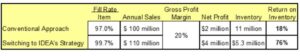
To be conservative, we assume a 10% sales increase. (In reality, we have never seen a sales lift so small.) This sales boost comes with less complexity; it is much easier to complete a sale rather than work around a shortage. No new operating expenses are needed to sell the products you have on hand. (Cost reductions due to less expediting, cross shipping and reduced interest expense due to having more cash are ignored here.) With only a 20% gross profit margin, a 10% sales lift adds 2% of sales to the bottom line. This would be appropriate for a distributor. If your company is a manufacturer, the improvement will be much greater, using these same assumptions.
The need for management intervention is reduced. Cash floods back into the company. Debt that seemed permanent can finally be repaid. Bottom line improvements are bigger every year, as gross profits increase much faster than operating expenses rise. New profits and inventory savings can be plowed back into expansions and acquisitions. Shippers’ Buffer strategy is a powerful growth engine. Don’t creep ahead, leap ahead.